Method
Transport
RW3D simulates the key transport processes in porous media: advection, dispersion, and diffusion. These are modeled using the Random Walk Particle Tracking (RWPT) scheme described in the section Random-Walk Particle-Tracking.
In the following sections, we outline the interpolation schemes and available options for simulating particle motion.
Warning
Concentration versus Total Density
For practical purposes, RW3D’s core algorithm solves the motion in time and space of the total density of a solute (\(\rho\)), which is related to concentration by the porosity and the retardation factor: \(\rho = \phi \times R \times c\).
This is something to remember when designing the particles injection in your input file.
If read_concentration_file is the specified injection type (type_inj), the code will internally convert the concentration values to total densities.
For all other injection types, the convertion should be done by the user, if needed.
This has no incidence on the outputs of the code, which are expressed in terms of mass fluxes (e.g., for (C)BTCs) and number of particles (e.g., for plume snapshots). If concentration values has to be estimated from the outputs, the user should convert local particle densities reflecting total densities (from plume snapshots) to concentrations.
A future release of the code will include an option to compute concentration fields.
Advective Motion
RW3D uses fluxes defined on an Eulerian grid. For each spatial direction, the Darcy flux \(\mathbf{q}\) must be specified at the faces of each finite-difference cell (see Figure Fluxes crossing the faces of a finite-difference cell.).
To compute the flux at the particle location, \(\mathbf{q}_p \; [L \, T^{-3}]\), RW3D applies interpolation schemes described in Flux interpolation. A simple linear interpolation has been shown to be consistent with the finite-difference formulation of the flow equation and ensures local mass conservation [Pol88].
The particle velocity \(\mathbf{v}_p(\mathbf{x}_p) \; [L \, T^{-3}]\) is then computed by scaling the interpolated flux by the local porosity or water content, \(\phi \; [-]\):
Unless otherwise noted, all parameters are specified or evaluated at the particle location \(\mathbf{x}_p\).
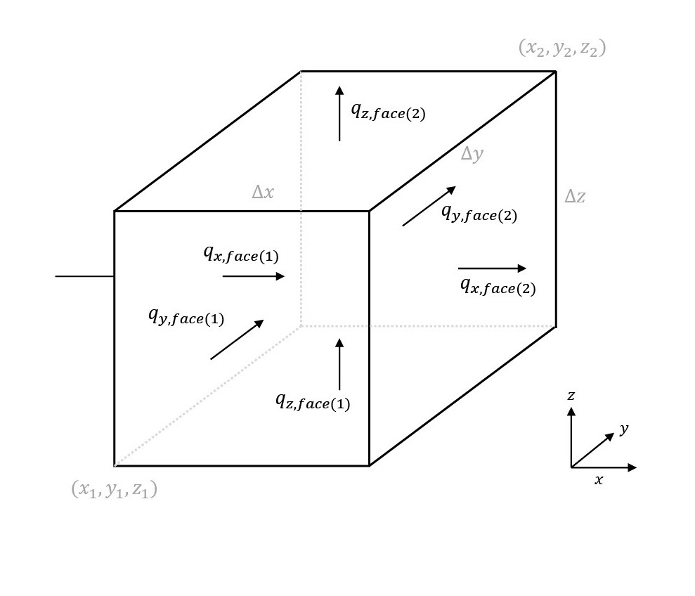
Fluxes crossing the faces of a finite-difference cell.
RW3D provides two options for simulating advective particle motion, i.e., the displacement due to advection during a time step \(\Delta t\), denoted \(\Delta \mathbf{x}_{p,\text{adv}}\):
Eulerian: Standard random-walk using Eulerian integration of the velocity:
(2)\[\Delta \mathbf{x}_{p,\text{adv}} = \int v_p(\tau) \, d\tau \approx v_p(t) \, \Delta t\]Exponential: Pollock’s method for integrating velocity in finite-difference flow models:
(3)\[\Delta \mathbf{x}_{p,\text{adv}} = \frac{v_{p,i}(t)}{A_i} \left( \exp(A_i \, \Delta t) - 1 \right)\]where:
\(A_i = \dfrac{v_{i,\text{face}(2)} - v_{i,\text{face}(1)}}{\Delta x_i}\)
\(v_{i,\text{face}(j)} \; [L \, T^{-3}]\) is the velocity in the \(i\)-th direction at the \(j\)-th face of the cell
\(\Delta x_i \; [L]\) is the cell size in the \(i\)-th direction
The exponential scheme provides a more accurate integration of velocity in regions with strong gradients and is particularly useful in heterogeneous domains.
Flux interpolation
Subsurface systems are inherently heterogeneous and often characterized by abrupt changes in soil and geological materials. Physical properties of grid-based flow solvers used under heterogeneous conditions are parameterized at a series of discrete points, which generates discontinuities in output parameters (e.g., velocities) that are subsequently used to solve transport. Yet, the RWPT algorithm requires smooth transitions in the water front in order to preserve local solute mass conservation. RW3D uses interpolation schemes to deal with discontinuities in the veocities and in the dispersion tensor.
To estimated the advective motion of the particle, the flux in the i-th direction is estimated using the following linear interpolation:
where \(xc_{i,face(1)}\) is the i-th coordinate of the first face of the cell hosting the particle.
If dispersion is accounted for, the local flux in the i-th direction used to calculate the random motion of the particle is estimated using the following trilinear interpolation scheme:
where:
\(F_i\) is the relative location of the particle within a cell defined as \(F_i = (x_{p,i}-xc_{i,face(1)})/\Delta i\)
\(q_{i,node(j,k,l)}\) is flux in the i-th direction at the node {j,k,l}
Time discretization
The appropriate determination of the time step between two particle jumps is essential for the RWPT method to properly solve the ADE. In general, the smaller the time step, the better.
The choice in this time step determination is left to the user. The time step (\(\Delta t\)) can be made constant (constant_dt option). This has to be used with caution.
To gain in efficiency and insure a good representation of key processes, we implemented few methods, based on characteristic times, that allows a generally satisfactorily estimation of the time step size while preserving computational efficiency. Time steps can take in consideration the advective characteristic time (\(t_{c,adv} \; [T]\)), the dispersive characteristic time (\(t_{c,disp} \; [T]\)), the reactive characteristic times (\(t_{c,kf} \; [T]\), \(t_{c,kd} \; [T]\)) and the mass transfer characteristic time (\(t_{c,mt} \; [T]\)). At each time step, the characteristic times are evaluated for each particle of the plume and the more restrictive is considered. The new time step is then estimated by multiplying the selected characteristic time by a constant:
The multiplier \(\text{Mult} \; [-]\) is specific to each considered process (mult_adv, mult_disp, mult_kf, mult_kd, mult_mt). Typically, the multiplicative inverse of the multiplier represents the number of particle jumps in a cell before the effect of the considered process is significantly modified.
We then advise to always keep \(\text{Mult}<1\) and to lower the values as much as sharp interfaces are simulated in order to minimize errors when particles jumps from a cell to another.
If many processes are simultaneously simulated (as it often occurs), the time step can be evaluated from advection only by selecting the constant_move option (here again, to be used with caution) or from all processes by selecting the optimum_dt option.
For the latter, the smaller time step will be considered.
In some case, considering the more restrictive characteristic time over the entire plume of particle can lead to impractically small time steps. This is required to properly simulate fast local processes, e.g., in case of high velocity zones near extraction wells.
However, if the solution near these more demanding zones is less relevant for the user, we provide an option to relax the time step. The coefficient dt_relax allows to consider only a given less restrictive portion of the characteristic times of the plume.
For example, if dt_relax is fixed to 0.9, only the less restrictive 90% of characteristic times are considered in the time step evaluation. The 10% shorter characteristic times (e.g., associated to the 10% fastest particles) will be disregarded.
The characteristic times are defined for each particle of the plume and at any discretized time as follow:
Advective characteristic time:
where \(\Delta_s \; [L]\) is the characteristic size of the cell where the particle is located:
\(\bar{v} \; [L \, T^{-3}]\) is the characteristic particle velocity estimated as:
Dispersive characteristic time:
where \(D_L \; [L^{2} \, T^{–1}]\), \(D_{TH} \; [L^{2} \, T^{–1}]\), \(D_{TV} \; [L^{2} \, T^{–1}]\) are the longitudinal, transverse horizontal and transverse vertical componenents of the dispersion tensor.
Reactive characteristic time:
In case a kinetic reaction is simulated:
where \(\max(k_f)\) refers to the maximum values of the kinetic reaction rates in a bimolecular reaction network.
In case a first-order decay reaction is simulated:
where \(k_d\) is the first-order decay associated to the particle.
Mass transfer characteristic time:
where:
\(\alpha\) is the mass transfer coefficient
\(\beta\) is the total capacity
Special cases
Unsaturated transport.
In case flow has been computed from an unsaturated flow solver (e.g., solving the Richard’s equation), transport equations remain identical and the water content field (homogeneous or heterogeneous, steady state or transient) can simply be considered as the porosity field.
Partially saturated cells.
Even using flow parameters from flow models solving the Darcy equation, cell can be partially saturated, e.g., in case of low water table in an unconfined aquifer. The saturation of each cell of the domain can be defined by the cell-by-cell head elevation. For the moment, in case particles located in a partially saturated cell and located above the head elevation, we consider vertical transport only by setting the horizontal fluxes to zero.
Change in cell thickness.
In case of horizontal motion to a cell with a different thickness after a time step \(\Delta t\), the relative local z-coordinate of the particle previous of the jump is preserved. The new particle location in z (\(z_{p}\)) is then corrected as follow:
where:
\(t\) and \(t + \Delta t\) refers to time before and after the horizontal jump in another cell, respectively
\(z_{c,bot}\) and \(z_{c,top}\) are the bottom and the top elevation of the cell
Backward particle tracking
To track particle in the backward direction, a.k.a. upstream, simply inverse the velocity field by setting the multiplier associated to the flow field to -1. No particular modification is made to the transport code. Note that setting up backward particle tracking accounting for dispersion does not provide a deterministic characterization of the plume origin, and should be done with cautious.
Reactions
RW3D solves a range of reactions, which are described below. We refer to the related reference for details about the method for solving such reactions using particle tracking techniques.
First-order decay networks
The transport equations governing the behavior of network reactions is given by a set of advective-dispersive equations coupled with first-order reactions:
where:
the ith-equation represents the mass balance of the ith species
\(n_s\) is the number of the species involved
\(\theta \; [-]\) is the porosity of the media
\(q \; [L \, T^{-1}]\) is the Darcy velocity vector
\(D \; [L^{2} \, T^{–1}]\) is the dispersion tensor
For any given species i:
\(c_i \; [M \, L^{–3}]\) is the concentration in the liquid phase
\(k_i \; [T^{–1}]\) is the first-order contaminant destruction rate constant
\(y_{ij} \; [M \, M^{–1}]\) is the effective yield coefficient for any reactant or product pair
These coefficients are defined as the ratio of mass of species i generated to the amount of mass of species j consumed.
RW3D solves this network by estimating the probability for a particle at a given state (i.e., species) at a given time to turn into another species after a given time step. The derivation, validation and application of the method is presented in Henri and Fernàndez-Garcia [HFG14].
Bimolecular reaction networks
RW3D is solving few types of bimolecular reactions. The reactive transport of such systems is given by:
where:
\(c_i \; [M \, L^{–3}]\) is the solute concentration of each species \(i\)
\(\theta \; [L^2 \, L^{-2}]\) is the water content
\(\mathbf{u} \; [L \, T^{-1}]\) is the pore water velocity
\(r(c_A, c_B)\) is the total rate of product creation via reaction and source
For instance, for a \(A + B \to C\), this reaction term is \(r(c_A, c_B) = -k_f c_A c_B\), where \(k_f \; [L^{2} \, M^{-1} \, T^{-1}]\) is the reaction rate coefficient.
For the moment, RW3D is solving the following bimolecular reactions:
0 product: \(A + B \to 0\)
1 product: \(A + B \to C\)
2 products: \(A + B \to C + D\)
In this package, these reactions can be associated to first-order reactions of the form:
0 product: \(A \to 0\)
1 product: \(A \to C\)
2 products: \(A \to C + D\)
Note
How to solve bimolecular reactions using RWPT?
The particle-based method used here simulates bimolecular reactions through probabilistic rules of particle collisions and transformation, as described by Benson and Meerschaert [BM08].
To illustrate the method, let’s consider a reaction \(A + B \to C\). For this reaction to take place, a A particle should be close enough to a B particle, so they can interact. Under natural, not well-mixed conditions, this process is controlled by the distance that a particle might diffuse or hydro-dynamically disperse, especially in the transverse direction to flow. Let’s assume two independent particles A and B, with initial locations \(x_t^A\) and \(x_t^B\), respectively. After a small time-step \(\Delta t\), the particles have moved to new positions, \(x_{t+\Delta t}^A\) and \(x_{t+\Delta t}^B\), respectively, with \(dx^A\) and \(dx^B\) is the actual displacement of each particle during \(\Delta t\). The probability that the two particles will occupy the same position, after \(\Delta t\), is given by:
(15)\[\begin{split}\begin{split} P\left(x_{t+\Delta t}^A = x_{t+\Delta t}^B \right) & = P\left( x_t^A+dx^A=x_{t+\Delta t}^B+dx^B \right) \\ & = P\left(dx^A-dx^B = x_{t+\Delta t}^B-x_{t+\Delta t}^A \right) \\ & = P\left(D=s\right) = P\left(D-s=0\right), \end{split}\end{split}\]where:
\(D=dx^A-dx^B\) is the relative displacement of the two particles
\(s=x_t^B-x_t^A\) is the initial separation distance
We assume that the two particles will be in contact (and react) if \(D\) is equal to \(s\) and the final displacement, \(D-s\) is equal to 0. Benson and Meerschaert [BM08] define the encounter density function \(v(s)\) as the density of \(D\). Now, assuming that the movement of the particles during \(\Delta t\) is symmetric, then for the case of B particles, \({dx}^B\) is identically distributed with \(-dx^B\), and since the displacements \(dx^A\) and \(dx^B\) are independent, \(D\) is identically distributed with \(dx^A+dx^B\). \(v(s)\) can then be considered as the sum of two independent random variables \(dx^A\) and \(dx^B\), which is known to be equal to the convolution of the two densities. Defining \(f_A(x)\) and \(f_B(x)\) as the densities of \(dx^A\) and \(dx^B\) (i.e., the densities of the motions away from the current positions \(x_t^A\) and \(x_t^B\)), we can write the following convolution equation:
(16)\[v(s)=\int{f_A(x)f_B(s-x)dx}.\]In RW3D, both \(f_A(x)\) and \(f_B(x)\) are considered as Gaussian densities to represent the mechanical dispersion of particles.
The probability density that a pair of particles A and B react is then given by:
(17)\[P\left(react\right) = k_f\times\Delta t\times m_p\times v(s)\]where \(m_p\) [M] is the mass of a particle.
The reaction probability P(react) is finally compared with a random number that is uniformly distributed between 0 and 1. If the probability of the reaction is larger than the random number, the two reactant particles are converted to a product particle. The location of the product particle is considered to be half-way between the two reactant particles.
Linear Sorption
Linear instantaneous sorption, i.e., retardation, is simply solved by scaling the advective flux:
where:
\(c\) \([g.m^{-3}]\) is the solute concentration
\(\phi\) is the effective porosity
\(\mathbf{D}\) is the dispersion tensor
\(R_i\) is the i-th species specific retardation factor
Multirate Mass Transfer
What is Multirate Mass Transfer?
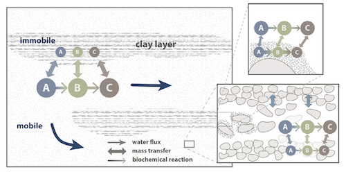
Illustration of reactions and mass transfer between the mobile and a series of immobile spheres.
The presence of stagnant water in micro- and meso-pores at the grain scale, as well as the inclusion of low-permeability zones at the field scale, often leads to the conceptualization of porous media as comprising two distinct regions:
a mobile region, where advection and dispersion dominate transport, and
an immobile region, where transport is primarily diffusion-limited.
Mass exchange between these regions occurs due to concentration gradients, allowing solutes initially present in the mobile domain to diffuse into the immobile zone, where they may become temporarily trapped and subsequently released over time.
This dual-domain conceptual model has gained significant attention for its ability to reproduce highly asymmetric concentration profiles observed in field studies [].
While early mass transfer models typically employed a single mass transfer coefficient to characterize exchange between mobile and immobile zones [], this approach has shown substantial limitations in predicting long-term solute behavior []. The inherent mineralogical heterogeneity of natural soils and the complex spatial variability of aquifer properties result in a spectrum of mass transfer processes occurring over multiple time scales—phenomena that cannot be adequately captured by a single coefficient.
To address this, the multirate mass transfer (MRMT) model introduced by incorporates multiple immobile domains, each characterized by distinct mass transfer coefficients and porosities. By selecting appropriate parameter values, the MRMT model can simulate a wide range of diffusion scenarios, including diffusion into cylindrical, spherical, planar, and fractured media.
The MRMT model.
Parameters of the multirate mass transfer model are species specific. In theory, reaction can occur in the mobile and immobile domains with specific reaction parameters. So, we present equations considering theoretical reactions. In a general form, and associated to a multispecies reactive system characterized by a first-order decay network, the MRMT model is given by:
where:
\(c_{i0} \left[M\, L^{-3}\right]\) is the concentration of the i-th species in the mobile domain (denoted always by the subscript index \(k=0\))
\(c_{ik} \left[M\, L^{-3}\right]\), for \(k=1,...,N_{im}\), is the concentration of the i-th species in the k-th immobile domain
\(N_s\) is the number of species
\(N_{im}\) is the number of immobile domains
\(\phi_0 [-]\) is the porosity of the media in the mobile domain
\(\phi_{k} [-]\) for \(k=1,...,N_{im}\) is the porosity of the media in the k-th immobile domain
\(R_{i0}\ [-]\) is the retardation factor of the i-th species in the mobile domain, and
\(R_{ik} [-]\) is the retardation factor of the i-th species in the k-th immobile domain \((k=1,...,N_{im})\)
\(\mathscr{L}(c)\) is the mechanical operator of the mobile concentrations defined by:
where:
\(\mathbf{q} \left[L\, T^{-1}\right]\) is the Darcy velocity vector
\(\mathbf{D}\) is the dispersion tensor \(\left[L^{2}\, T^{-1}\right]\)
The first equation (MRMT) is actually the mass balance associated with any of the species involved in the network reaction system, and equation (MRMT2) describes the mass transfer of the i-th species between the mobile domain and the k-th immobile domain.
This mass transfer process is characterized by the apparent mass transfer coefficient \(\alpha_{ik} [T^{-1}]\), which is defined as
where \(\alpha^\prime_k\) is the first-order mass transfer rate coefficient between the mobile domain \((k=0)\) and the k-th immobile domain \((k=1,...,N_{im})\).
The right-hand-side of equation MRMT represents the destruction and production of the different species driven by first-order kinetic reactions, where:
\(k{}_{i\ell} \left[T^{-1}\right]\) is the first-order contaminant destruction rate constant associated with the i-th species and \(\ell\) domain
\(y{}_{ij} \left[M\, M^{-1}\right]\) is the effective yield coefficient for any reactant or product pair (i,j). It is a stoichiometric coefficient that is assumed constant for all domains. These coefficients are defined as the ratio of mass of species i generated to the amount of mass of species j consumed. The yield coefficients \(y{}_{ii}\) are equal to \(-1\) and represent the first-order decay of the i-*the species.
In our implementation, only aqueous concentrations can undergo chemical reactions, i.e., no reactions occur in the sorbed (immobile) phase.
Diffusion into different geometries
The multirate model offers the advantage of also simulating diffusion into spheres, cylinders, and layers. This is achieved by selecting appropriate values for the first-order rates and capacity coefficients [HG95]. More discussion about the modeling of diffusion into different geometries using RWPT can be found in Salamon et al. [SFernandezGarciaGomezHernandez06].
The series of these coefficients for the different geometries are shown in the following table:
Diffusion geommetry |
\(\alpha_j\) (for \(j=1,\dots,N_{im}-1\)) |
\(\beta_j\) (for \(j=1,\dots,N_{im}-1\)) |
\(\alpha_j\) (for \(j=N_{im}\) ) |
\(\beta_j\) (for \(j=N_{im}\) ) |
|---|---|---|---|---|
Layered diffusion |
\(\dfrac{(2j-1)^2\pi^2}{4}(D_a/a^2)_i\) |
\(\dfrac{8}{(2j-1)^2\pi^2}\beta_{tot}\) |
\(\dfrac{3\left(D_a/a^2\right)_i \left[ 1- \displaystyle\sum_{j=1}^{N_{im}-1}\frac{8}{(2j-1)^2\pi^2}\right]}{1- \displaystyle\sum_{j=1}^{N_{im}-1}\frac{96}{(2j-1)^4\pi^4}}\) |
\(\left[ 1 - \displaystyle\sum_{j=1}^{N_{im}-1} \dfrac{8}{(2j-1)^2\pi^2} \right]\beta_{tot}\) |
Cylindrical diffusion [1] |
\(r^2_{0,j}(D_a/a^2)_i\) |
\(\dfrac{4}{r^2_{0,j}}\beta_{tot}\) |
\(\dfrac{8\left(D_a/a^2\right)_i \left[ 1- \displaystyle\sum_{j=1}^{N_{im}-1}\frac{4}{r^2_{0,j}}\right]}{1- \displaystyle\sum_{j=1}^{N_{im}-1}\frac{32}{r^2_{0,j}}}\) |
\(\left[ 1- \displaystyle\sum_{j=1}^{N_{im}-1}\frac{4}{r^2_{0,j}}\right]\beta_{tot}\) |
Spherical diffusion [2] |
\(j^2\pi^2(D_a/a^2)_i\) |
\(\dfrac{6}{j^2\pi^2}\beta_{tot}\) |
\(\dfrac{15\left(D_a/a^2\right)_i \left[ 1- \displaystyle\sum_{j=1}^{N_{im}-1}\frac{6}{j^2\pi^2}\right]}{1- \displaystyle\sum_{j=1}^{N_{im}-1}\frac{90}{j^4\pi^4}}\) |
\(\left[ 1- \displaystyle\sum_{j=1}^{N_{im}-1}\frac{6}{j^2\pi^2}\right]\beta_{tot}\) |
Sink
Sink-cells
The mass transfered to a sink during a time step is estimated cell by cell. For each time step, the number of particles extracted in a sink cell (n_{p_{s,tot}}), i.e., a cell affected by at least one sink and for which the total flux into sinks (\(Q_{s,tot}\)) is larger than 0, is given by:
where:
\(n_{p_{c}}\) is the number of particle located in the sink cell
\(n_{p_{s,tot}}^*\) is the residual number of particle to be extracted from the previous time step
\(S_s\) is the total sink strength, which is estimated by:
where \(V_{s,tot} [L^3]\) is the total volume of water extracted by all sinks located in the cell, and \(V_{c} [L^3]\) is the volume of water in the cell.
These volumes are calculated as:
where \(Q_{s,i}\) is the volume of water extracted by each sink i located in the sink cell.
where \(\Delta z^*\) is the saturated thickness of the cell.
The number of particles to be extracted by each sink i located in this sink cell (\(n_{p_{s,i}}\)) is then given by:
where:
\(n_{p_{s,i}}^*\) is the residual number of particle to be extracted by the sink i from the previous time step
\(S_i\) is the relative sink strength, which is estimated by:
where \(V_{s,i} [L^3]\) is the volume of water extracted by the sink-cell i.
Equations npart_all_sink and npart_sink_i does not produce necessarly an integer (i.e., entire number of particles). \(n_{p_{s,tot}}^*\) and \(n_{p_{s,i}}^*\) are the differences between the number of particle actually extracted (integer) and the calculated number (real). These residuals are added over each time step interation until reaching an entire particle, which will then be removed.
The distribution of particles among all sinks affecting in a single sink cell is favoring the sink requiring the larger number of particle. In case the same number of particles is required, the sink in which the particle will assigned to is selected randomly.
Wells
Mass extraction by pumping wells is implemented in two ways. First, wells can be considered as a sink cell. In this case, the convergence of travel paths toward the actual well location is not considered. Particles will be extracted uniformly in the sink-cell following the weak sink-cell extraction algorithm, as described in the section Sink-cells.
Particle extraction in wells can also be more explicitly simulated by estimating the path of particles toward a well located in a cell. In case of weak sink due to the presence of an extraction well, using the simple interpolation scheme described in Advective Motion fails to reproduce the increase of velocity the closer the well is and to identify if a particle should be captured by the well or leave the cell from the face where an outflow exists. To solve these issues, we use the approximate analytical solution presented in Zheng [Zhe94]. The components of the velocity of a particle located in a cell affected by a well extraction can then be estimated as:
where:
\(x_{w}\) and \(y_{w}\) are the coordinates of the well
\(Q_{w} [L^3/T]\) is the volumetric extraction flux of water extracted by the well
\(a [-]\) is the horizontal anisotropy of the hydraulic conductivity.
For the moment, our implementation does not account for this potential anisotropy in the hydraulic conductivity. The coefficient a is then fixed to 1.0.
Note that the well is here supposed to fully penetrate each well-cell and that the well could be located at any place horizontally in the cell (does not have to be located at the center).
The particle transport is terminated once it moves within the radius of the well (\(r_{w}\)), which has to be specified.
Outputs
The code provides options to:
Record particle arrivals to a series of observation objects (sinks, control planes, observation wells, and/or registration lenses) by generating Breakthrough curves, Cumulative breakthrough curves, full Plume history. Temporal moments of BTCs from wells and planes of arrivals to control planes and observation wells can also be provided.
Capture and analyze the plume of particle by providing Plume snapshots, Particle paths, and by computing Spatial Moments at specific times.
Plume snapshots
The location of all particles can be printed in a file at a series of user-defined time steps. The file will also provide the mass, the zone, the specie and the ID of the particles.
Tip
The generated csv files (if this is the chosen output format) can be directly imported into Paraview for 3D visualization. In Paraview, use the TableToPoint filter after importing your data.
You can also import together the series of csv files generated for each snapshot (at selected time) to generate an animation.
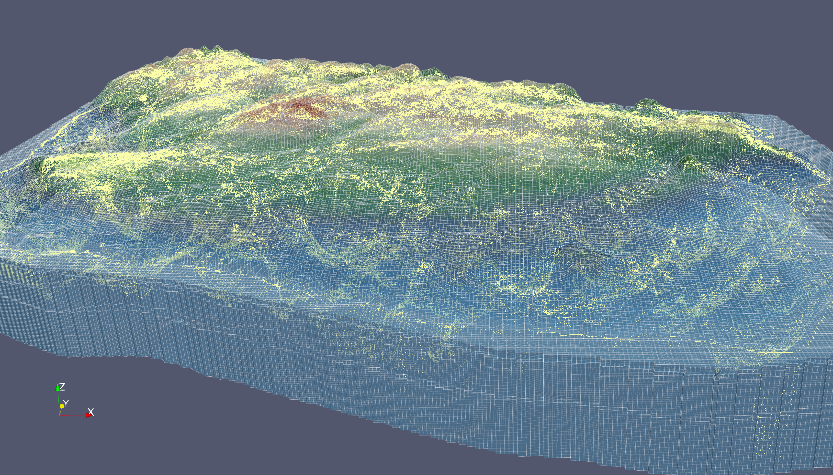
Example of a single plume snapshot visualized in Paraview.
Cumulative breakthrough curves
Mass arrival to observation objects can be recorded as cumulative breakthrough curves (CBTCs). CBTCs are simply obtained by adding particle mass at the time of their arrival and represent the total mass that has reached the observation object up to a given time. CBTCs are useful for assessing the completeness of transport (i.e., how much of the total injected or released mass has reached the observation point) and/or for comparing total mass recovery.
where \(F(t)\) is the cumulative mass that has passed the observation point up to time t.
Breakthrough curves
Mass arrival over time can be obtained under the form of breakthrough curves (BTCs), i.e, the evolution of mass fluxes over time (units M/T). BTCs are useful in showing how quickly and in what quantity particles reached an observation object over time, providing insight into transport dynamics such as advection and dispersion.
where \(M(t)\) is the mass flux at time t.
Particle tracking simulations produce discrete arrival times of particles at an observation object. A reconstruction process is then needed to convert particle arrivals into concentrations. This reconstruction process is normally seen as the main disadvantage of PTMs. RW3D uses Kernel density estimator (KDE) to transform these discrete events into a continuous, smooth estimate of the breakthrough curve, which can be more interpretable and suitable for analysis.
Kernel Density Estimation
Given a sample of particle travel times \(\{t_1, t_2, \dots, t_n\}\), the kernel density estimate of the underlying probability density function \(f(x)\) is defined as:
where:
\(n\) is the number of particles reaching the observation object,
\(K(\cdot)\) is a kernel function (e.g., Gaussian),
\(h\) is the bandwidth (smoothing parameter).
Bandwidth Selection
In kernel density estimation, the bandwidth is a critical parameter that controls the degree of smoothing applied to the data. A small bandwidth results in a curve that closely follows the individual particle arrival times, potentially capturing noise and producing a jagged breakthrough curve. Conversely, a large bandwidth oversmooths the data, potentially obscuring important features such as peaks or multimodal behavior. Selecting an appropriate bandwidth is essential for accurately representing the underlying transport dynamics.
Plugin Method
The method proposed by Engel, Herrmann, and Gasser (1994) provides an iterative, data-driven approach to selecting the optimal bandwidth for kernel density estimation (KDE), particularly when estimating both densities and their derivatives.
The optimal bandwidth minimizes the Mean Integrated Squared Error (MISE):
However, the optimal bandwidth depends on unknown quantities such as \(f''(x)\). The Engel-Herrmann-Gasser method estimates these quantities from the data and refines the bandwidth iteratively.
Iterative Procedure
Start with an initial pilot bandwidth \(h_0\).
Estimate the density and its derivatives using \(h_0\).
Plug these estimates into the formula for the optimal bandwidth.
Update the bandwidth and repeat until convergence.
This method is particularly effective for accurate estimation of density derivatives and is more robust than simple rule-of-thumb or fixed plug-in methods.
Plume history
This option proposes to record all arrivals to any observation object by providing the following particle information in an ascii or binary file:
ID: particle ID assigned at the injectionX-BIRTH,Y-BIRTH,Z-BIRTH: coordinates of the recorded particle at the time of its injectionIX-BIRTH,IY-BIRTH,IZ-BIRTH: index of the cell where the particle was injectedX-REG,Y-REG,Z-REG: coordinates of the recorded particle at the time of arrival to the observation objectIX-REG,IY-REG,IZ-REG: index of the cell where the particle was registrated in the observation objectREGISTRATION_NUMBER: index of the registration lense where the particle has been recorded, if registration lenses are used. The values 0 will be displayed otherwise (in case of arrival to sinks or other observation object)TRAVEL_TIME: Time of the particle arrival to the observation objectSINKTYPE: Sink name, or observation well name,SPECIE: Name of the chemical species of the particle
Particle paths
With this option, the path (together with key properties) of a given or all particles will be printed at any time or following a given temporal frequency.
Spatial Moments
Spatial moments are statistical measures used to characterize the distribution of a solute plume in space. In RW3D, the first and second spatial moments are computed from the particle distribution to quantify the plume’s location and spread over time.
First spatial moment The first spatial moment represents the center of mass (or centroid) of the plume in each spatial direction:
where:
\(X_g^i\) is the centroid in the \(i\)-th direction
\(m_{p_k}\) is the mass of particle \(k\)
\(x_{p_k}^i\) is the position of particle \(k\) in the \(i\)-th direction
\(R_k\) is a weighting factor (e.g., accounting for residence time or detection probability)
Second spatial moment The second spatial moment quantifies the spread or variance of the plume, and is used to compute the covariance matrix of the particle distribution:
where:
\(M^{i,j}\) is the covariance between the \(i\)-th and \(j\)-th spatial directions
The second term subtracts the product of the first moments to center the distribution
Applications in Contaminant Transport Modeling
Spatial moments are powerful tools for analyzing solute transport:
The first moment tracks the advective movement of the plume, indicating how far and in which direction the contaminant has traveled.
The second moment characterizes dispersion and spreading, helping to quantify how the plume evolves over time due to heterogeneity, diffusion, and mechanical dispersion.
The covariance matrix derived from second moments can reveal anisotropy in spreading, such as preferential flow paths or barriers.
Temporal moments of BTCs from wells and planes
RW3D computes temporal moments from particle arrival times to characterize the shape and timing of breakthrough curves (BTCs). These moments are calculated directly from the arrival times of particles recorded at a given observation point or control plane.
The following statistical moments are computed:
Non-central (raw) moments
The first four non-central moments of the particle arrival times \(t_p\) are computed as:
where:
\(t_{p_k}\) is the arrival time of particle \(k\)
\(N\) is the total number of particles
\(\alpha_n\) is the \(n\)-th raw moment
Central moments
The central moments are then derived from the raw moments using standard transformations:
These correspond to:
\(\mu_1\): Mean arrival time
\(\mu_2\): Variance of arrival times
\(\mu_3\): Third central moment (used for skewness)
\(\mu_4\): Fourth central moment (used for kurtosis)
Skewness and kurtosis
The skewness and excess kurtosis of the breakthrough curve are computed as:
If the variance \(\mu_2\) is zero (i.e., all particles arrive at the same time), skewness and kurtosis are set to zero, and a warning is issued.
Applications in Contaminant Transport Modeling
Temporal moments are valuable for:
Characterizing breakthrough curves: They summarize the timing and duration of solute arrival in a compact form.
Estimating transport parameters: Moments can be used to infer effective velocity, dispersion coefficients, and retardation factors.
Quantifying tailing and non-Fickian behavior: Higher-order moments reveal asymmetry and long-term persistence in solute arrival.